The Power of Multitask Learning

One of the fundamentals of the human learning process is that multiple tasks are learned in parallel, and not as independent tasks. Throughout this process, knowledge and experiences acquired in one task, are shared and transferred to the others. This general idea has been adopted in machine learning (ML) as well and has been shown to be beneficial in terms of learning efficiency and prediction accuracy. This subfield of ML is referred to as Multi-Task Learning (MTL).

In this post we will familiarize ourselves with the general concept of MTL and demonstrate the power of MTL compared to Single-Task Learning (STL) approaches, over the problem of multidimensional time-series forecasting.

Motivation

Multitask learning is an approach in which multiple learning tasks are solved simultaneously, in order to improve the generalization performance of the single tasks, by leveraging the information contained in the training signals of other tasks. In other words, MTL aims to improve the accuracy of task-specific models, by utilizing similarities and relations between the different problems.

In some cases, our main goal is indeed to optimize the model’s performance over a set of tasks, however, typically in ML, we are only interested in optimizing for a single task (e.g. STL regression/classification frameworks). Even if that is the case, it has been shown that adding additional learning problems (often referred to as auxiliary tasks), will allow us to improve upon our main (original) task. In the latter, MTL can be viewed as a regularization method, in which regularization is induced by optimizing the model’s performance over all tasks.

Background

Many approaches have been developed in order to learn multiple tasks simultaneously (see e.g. [1], [2]). Perhaps the most common approaches nowadays use (deep) neural networks (NN), in which information is transferred across tasks through hard/soft parameter sharing. The more “classical” ML approaches use linear models and kernel methods (and sometimes involves Bayesian approaches). In general, we can divide these approaches into two classes:

• Feature learning approaches, which involve either feature selection across tasks through norm regularization, or feature transformation (e.g. parameter sharing in NNs).
• Task relation learning approaches, in which task relations are used to enforce similarities between related tasks. These relations are assumed to be known a priori, or learned directly from the data.

To keep things simple, we are going to focus on a simple (and commonly used) linear approach, which induces cross-task feature selection (i.e. feature learning approache).

Problem Formulation

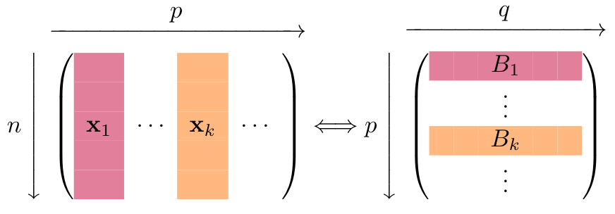
In the general case, each task might consist of its own training data, however, in many cases, the same set of explanatory variables, \(X\in\mathbb{R}^{n\times p}\), is used to model the different target variables, \(\textbf{y}_i \in \mathbb{R}^n\) for \(i=1,...,q\). For example, an on-demand transportation company may attempt forecasting demand and supply in different time frames and geographic locations. The general task of modeling multiple responses using a joint set of covariates can be expressed using multivariate regression (MR), or multiple response regression — a generalization of the classical regression model to regressing \(q > 1\) responses on \(p\) predictors. The multivariate regression model is given by,

\[Y=XB+E\]

where \(Y\in\mathbb{R}^{n\times q}\) denote the response matrix, \(B\) is a \(p \times q\) regression coefficient matrix, and \(E\) is an \(n \times q\) error matrix. A naive approach to the MR problem is to apply one of the STL methods, i.e. lasso, ridge, etc. to each of the \(q\) tasks independently. However, in many cases, the different problems are related, and this oversimplified approach fails to utilize all the information contained in the data.

Shared Information

The multivariate regression framework naturally induces a group structure over the coefficient matrix, in which every explanatory variable, \(\textbf{x}_{j}\) for \(j = 1, ..., p\), corresponds to a group of \(q\) coefficients, \(B_j\).

The multivariate regression framework naturally induces a group structure over the coefficient matrix.

One popular and simple approach for MTL that utilized this group structure, is the group lasso (see e.g. [3], [4]), in which a lasso-like penalty is placed over pre-defined groups of coefficients (this penalty is also referred to as \(L_1/L_2\)-penalty). The group lasso objective function is given by,

\[\arg\min_{B} \Vert Y-XB\Vert_F^2 + \lambda \sum_{j=1}^p \Vert B_j\Vert_2\]

where \(\lambda\) is a regularization parameter \(\Vert \cdot \Vert_F\) is the Frobenius norm, and \(B_j\) is the \(j\)th row of \(B\). The \(L_1/L_2\)-penalty encourages coefficients within the same group to share a similar absolute value, and essentially perform cross-task variable selection, in which a variable (corresponds to a row in \(B\)) is either selected or omitted from all tasks. Thus, this method allows us to learn a common sparsity structure, and to recover the joint support — the set of variables that are relevant for all tasks.

Next, we compare the results of applying the MTL approach of group lasso to the STL lasso approach (applied for each task independently).

Forecasting Taxi Rides

We use the Chicago Taxicabs dataset which includes taxi trips from 2013 to mid. 2017, reported to the City of Chicago. We utilize the Fourier series to model the periodic effects of our multivariate time-series, similar to [5], [6]. For a seasonal period \(P\), this involves generating \(2\cdot N_p\) features of the form,

\[X_P(t)=\left\{\cos\left(\frac{2\pi nt}{P}\right), \sin\left(\frac{2\pi nt}{P}\right)\right\}_{n=1,...,N_p}\]

In addition, we incorporate covariates for the modeling of a piecewise linear trend. These transformations shift the multivariate time-series problem into a feature space with \(p = 70\), where the linear assumption is appropriate.

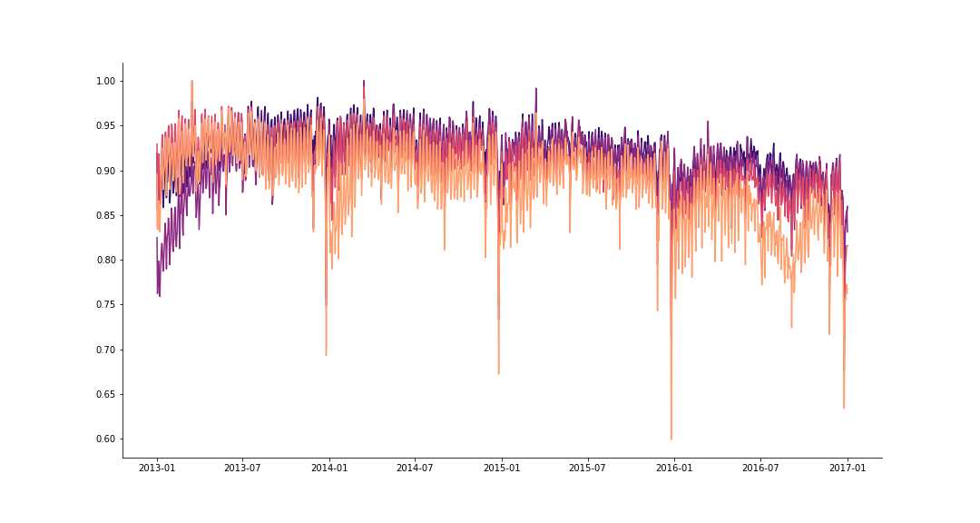
The daily number of rides (scaled) for 4 Taxi vendors in Chicago.

We predict the future number of rides for 4 providers, using the simulated historical forecasts (SHF) approach of [5], for producing \(K=32\) forecasts at various cutoff points in the history. For cutoff \(k = 0, ..., K −1\), we use the first \(n_{train,k} = n_{start} +k \cdot 7\) days for training, and the next \(n_{test} = 7\) observations for the test set. We then evaluate the performance of the model by the mean squared error (MSE), averaged over all tasks,

\[\text{MSE}_k=\frac{1}{n_{test}}\cdot\frac{1}{q}\sum_{t\in T_k}\sum_{j=1}^{q}(y_{j,t}-\hat{y}_{j,t})\]

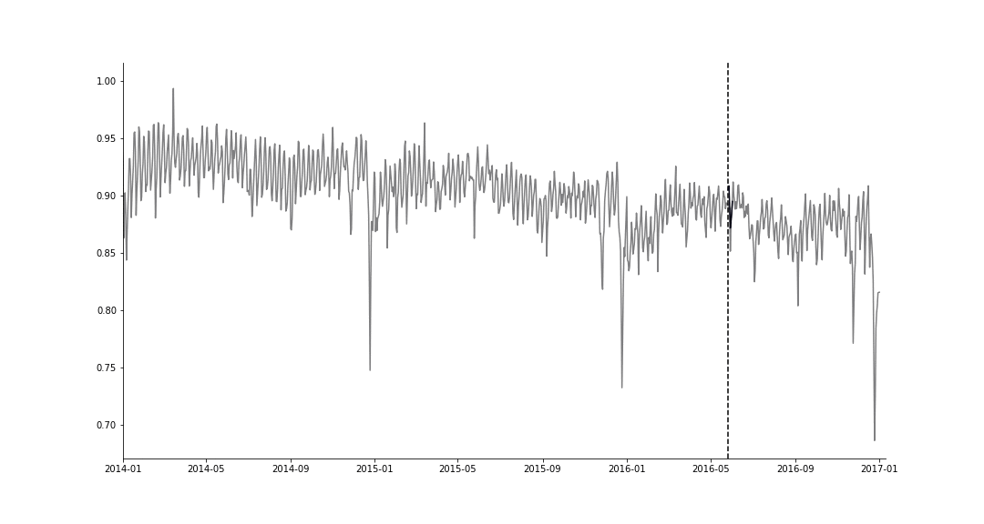
SHF example for a single task.

For this data, we get a 2.2% decrease in MSE (in favor of the MTL approach). Although the boost in performance is not mind-blowing, it’s not bad considering we have only tweaked the penalty term in the objective function, to encourage shared sparsity structure between tasks.

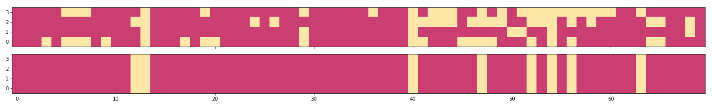
The sparsity structure for the STL lasso (top) and the MTL group lasso (bottom), at a single cutoff, with zero entries colored in yellow.

We’ve mentioned that the group lasso penalty produces the same sparsity structure across all tasks. The above plot shows the transposed coefficient matrices (rows for tasks and columns for variables), \(B^T\), for the STL lasso (top) and the MTL group lasso (bottom), with zero entries colored in yellow. We can see that the sparsity structure is indeed shared among tasks in the MTL model, whereas each STL model has its own sparsity structure.

Conclusion

In this post we have introduced the concept of multitask learning and demonstrated it’s power through a simple example of multidimensional time-series forecasting, using group lasso. This model, essentially assumes that the error terms for the different tasks are independent, and that the within-group similarities arise solely through a joint sparsity structure. There are other models that allow one to capture more complex relationships and relatedness among tasks (see e.g. [7], [8]), but we will leave this for future posts.

The code for producing all results and visualizations is available at my GitHub repo.

References and Further Readings

[1] Zhang, Yu, and Qiang Yang. “A survey on multi-task learning.” arXiv preprint arXiv:1707.08114 (2017).
[2] Ruder, S., 2017. An overview of multi-task learning in deep neural networks. arXiv preprint arXiv:1706.05098.
[3] Yuan, Ming and Yi Lin (2006). “Model selection and estimation in regression with grouped variables.” In: Journal of the Royal Statistical Society: Series B (Statistical Methodology) 68.1, pp. 49–67.
[4] Obozinski, Guillaume R, Martin J Wainwright, and Michael I Jordan (2009). “High-dimensional support union recovery in multivariate regression.” In: Advances in Neural Information Processing Systems, pp. 1217–1224.
[5] Sean J. Taylor, Benjamin Letham (2018) Forecasting at scale. The American Statistician 72(1):37-45
[6] Andrew, Harvey C and Shephard Neil (1993). “Structural time series models.” In: Econometrics. Vol. 11. Handbook of Statistics. Elsevier, pp. 261–302.
[7] Rothman, A.J., Levina, E. and Zhu, J., 2010. Sparse multivariate regression with covariance estimation. Journal of Computational and Graphical Statistics, 19(4), pp.947-962.
[8] Navon, A. and Rosset, S., 2018. Capturing Between-Tasks Covariance and Similarities Using Multivariate Linear Mixed Models. arXiv preprint arXiv:1812.03662.

---